Why JEPA Beat ImageNet Pretraining for Spacecraft Pose

A chaser spacecraft trying to dock with an uncooperative target has one camera, no time to phone home for help, and has to answer a hard question dozens of times a second: where exactly is that object, and which way is it facing? That's the 6-DoF pose problem — three numbers for position, three or four for orientation depending on parameterization — and it needs to run in real time on hardware modest enough to fit on a satellite bus.

There are two established ways to solve it. Geometric solvers detect keypoints in the image and hand them to a PnP algorithm, usually wrapped in RANSAC to survive outliers, which triangulates a pose against a known 3D model. This is accurate, but it's iterative and depends on having a precise CAD model of the target — something you often don't have for an unfamiliar or uncooperative satellite. Direct regression networks skip all of that and map pixels straight to a pose in a single forward pass. That's fast, but historically less accurate, and the reason turns out to be about what these networks are trained to care about, not their architecture. That mismatch is where SPACE-HOP starts.

The problem with teaching a network to "see clearly"

Most pretraining objectives — ImageNet classification, autoencoder-style reconstruction — are ultimately asking a network to get good at describing what a pixel grid looks like. That's fine for a lot of vision tasks. It's actively counterproductive here, because orbital imagery is a strange environment: no atmosphere to soften anything, one hard directional light source, knife-edge shadows, and reflective panels throwing blown-out highlights that shift completely with viewing angle.

A network optimized to minimize pixel error will happily learn to predict exactly where the glare falls, because that's an easy, high-signal target to fit. The problem is that signal disappears the moment the sun angle changes. The network hasn't learned anything about the spacecraft's shape — it's learned to describe this one photograph. What we actually want is a representation that stays stable when the lighting doesn't: a solar panel edge should look roughly the same to the network whether it's lit or in shadow. That's a geometric prior, not a photometric one, and no amount of getting better at pixel reconstruction produces it — reconstruction is precisely the objective that rewards the photometric detail we want the network to ignore.

Learning by filling in the gaps, not the pixels

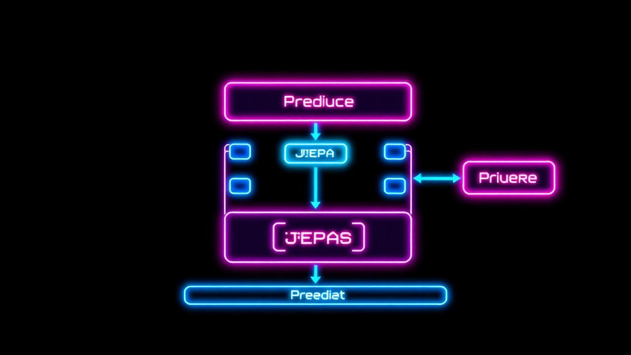
Joint-Embedding Predictive Architectures (JEPA) take self-supervision from a different angle. Instead of asking "given this partial image, reconstruct the missing pixels," JEPA asks "given this partial image, predict what the missing region's representation would be, according to a slowly-evolving version of yourself." Concretely: a context encoder looks at the visible patches, a target encoder — updated as an exponential moving average of the context encoder, so its output drifts slowly and stays stable — looks at the masked patches, and a lightweight predictor tries to guess the target encoder's output using only the context embeddings and a mask token. The loss lives entirely in embedding space. No pixel is ever reconstructed, no texture is ever scored.

This matters because embedding space is a far more forgiving place to be wrong about lighting, and a much less forgiving place to be wrong about structure. Two patches of the same antenna — one sunlit, one in shadow — can map to nearly identical embeddings if the network has learned to represent "this is an antenna joint" rather than "this pixel is bright." A pixel-reconstruction loss has no way to express that kind of abstraction, since it's graded pixel by pixel. An embedding-prediction loss can simply say: close enough, you got the geometry right, the shading doesn't matter.

We pushed this further with what we call keypoint-anchored masking. Standard JEPA masks patches more or less arbitrarily. We mask around the spacecraft's actual structural features instead — antenna tips, panel corners, docking interfaces, load-bearing vertices. The network has to predict the embedding of, say, an antenna tip using only patches that are spatially far away from it, with no local pixel correlation to lean on. The only way to succeed at that is to have built an internal model of how the whole rigid structure fits together, so that seeing three corners of a panel lets you infer the fourth.

The attention maps make the difference easy to see, not just measure. A standard supervised ViT backbone spreads its attention across the whole satellite body and often the background too — it's looking at everything indiscriminately. The JEPA-pretrained backbone concentrates sharply on the geometrically meaningful parts: corners, antennas, panel edges. It learned, without any supervision, to look where a human would look if asked to judge an object's orientation by eye.

Why regressing a rotation directly is a trap

Say you've got a great representation. You still have to turn it into an actual rotation, and this is where a second, less obvious problem shows up: rotations don't sit comfortably in Euclidean space, and every common way of parameterizing them has a failure mode. Euler angles gimbal-lock — you lose a degree of freedom at certain orientations, and the loss landscape develops singularities right where you least want them. Quaternions have antipodal ambiguity: q and −q represent the exact same rotation, so a naive loss function sees two "correct" answers on opposite sides of the space and can get pulled toward the unstable point in between. Continuous 6D rotation representations avoid both of those problems, but introduce their own — they're recovered via Gram-Schmidt orthogonalization, and if the network's raw output vectors ever drift near-collinear, that step's gradients explode.

The theoretically clean fix is to stop predicting a single rotation and instead predict a full probability distribution over SO(3) — the Matrix Fisher distribution is the natural choice, since it captures anisotropic uncertainty properly. The catch is that evaluating its normalizing constant requires an eigenvalue decomposition on every forward pass, which is fine in a research notebook and unworkable on a Jetson-class board doing real-time inference in orbit.

So we split the difference: approximate the distribution with a discrete grid, cheaply, and refine afterward. First figure out roughly where you are, then correct locally. This sidesteps every failure mode above — no angle parameterization to lock, no antipodal vectors to negate, and nothing reconstructed from raw continuous coordinates that could blow up. The coarse stage is just classification, about the most numerically boring, well-behaved thing you can ask a neural network to do.

Building an unbiased grid with the Hopf fibration

The obvious way to build a rotation grid — sweep Euler angles at fixed intervals — produces a badly non-uniform sampling: points bunch up near the poles and thin out near the equator, the same distortion you'd see on a Mercator map. For a classifier, that means some regions of rotation space get disproportionately fine resolution and others get coarse, arbitrary resolution, purely as an artifact of how you chose to parameterize things.

The Hopf fibration gives a way out. It's a map that takes the 3-sphere S³ — where unit quaternions, and therefore rotations, actually live — and decomposes it into a base S² sphere with a circle (S¹) attached at every point. Concretely, we scatter points evenly across the S² base using a Fibonacci lattice (a standard trick for spacing points uniformly on a sphere without clustering at the poles), then at each of those base points lay down a ring of evenly-spaced in-plane rotations. The result is a grid of anchor rotations spread uniformly across all of SO(3), with no directional bias baked in by the choice of coordinates. That matters a lot for a target as geometrically symmetric as a satellite bristling with panels and appendages.

Coarse, then fine: classify first, then nudge

Once the grid exists, the network's job splits into two linear heads sitting on top of the same [CLS] token. A classifier head scores every anchor rotation and picks the best match — an ordinary softmax-over-K-classes problem, trained with cross-entropy, as numerically tame as any ImageNet classifier. This gets you into the right neighborhood of SO(3), but a finite grid can only ever be so fine — even a dense one leaves a residual gap between the nearest anchor and the true orientation.

That's what the offset head is for. It predicts, per anchor, a small vector in the tangent space at that anchor — a local, linear approximation of how far and which way to nudge from there. We take the offset for whichever anchor the classifier picked and map it back onto the curved rotation manifold using the exponential map, the standard way to convert a straight-line tangent step into a proper rotation. Composing the anchor with this refinement gets sub-degree precision: the classifier handles the big, discontinuous decision of which general orientation this is, and the offset handles the small, smooth correction of exactly how far off the closest anchor was.

Translation gets separate treatment, since the problem there is different: predicting a 3D translation vector directly is scale-ambiguous, because a small close object and a large distant one can project to the same size in the image. We separate depth from lateral position and normalize everything against the 2D bounding-box crop before the network ever sees it, so the regression targets don't drift depending on how tightly or loosely the object happens to be cropped in a given frame.

What actually moved the needle

• ▸JEPA pretraining beat training a ViT-B from scratch with a reconstruction objective, on the identical downstream pipeline: 0.096 m translation error and 3.995° rotation error, versus 0.125 m and 6.143° — same architecture, same data, only the pretraining objective changed.
• ▸The classify-then-refine rotation head beat direct SE(3) regression on the same pretrained backbone by a wide margin: 0.096 m / 3.995° versus 0.173 m / 12.324° — more than a 3x improvement in rotation error from changing how the output is parameterized alone.
• ▸Deeper MLP heads and gated residual networks on top of the JEPA features gave no consistent improvement over a plain linear layer — a strong hint the backbone itself was already doing the hard work, and a simple readout was enough because the representation underneath was already geometrically organized.

The two-peaked error curve that tells on the spacecraft, not the model

Look at the rotation-error histogram on the real-image domains — Sunlamp and Lightbox — and instead of one clean peak near zero, there are two: one near 0° and a second near 180°. At first glance that looks like the model failing badly on a chunk of test cases. It isn't, or at least not primarily. The Tango spacecraft used in SPEED+ has real axial symmetry — certain orientations 180° apart produce images that are genuinely, visually almost indistinguishable, the way a symmetric coffee mug looks identical from the front whether the handle is hidden behind it or absent. The network isn't confused about geometry; the geometry itself is underdetermined by the image.

To pin down how much of this ambiguity actually lives inside the learned representation, rather than just showing up as noise in the final prediction, we built a diagnostic we call Jensen Gain. Take an image, apply a set of symmetry-preserving rotations to it, run the model on each, then rotate every prediction back into a shared reference frame. If the representation is truly symmetry-consistent, all those canonicalized predictions should collapse onto the same point — rotating the input and un-rotating the output should be a round trip that returns you exactly where you started. Any leftover spread after that round trip is dispersion the model itself introduced, not something you can blame on the input. Predictions scatter into two distinct clusters in symmetry-breaking cases and collapse into one tight cluster in stable ones. Sunlamp and Lightbox show measurably higher average Jensen Gain than the clean synthetic domain, which lines up with the intuition: harsh, directional real-world lighting makes the already-thin visual cues that break symmetry even thinner.

Where this leaves us

Trained entirely from scratch on SPEED+ — no external pretraining, no test-time adaptation, no borrowed ImageNet weights — SPACE-HOP lands within striking distance of regression baselines built on larger pretrained backbones, and stays competitive with PnP-based solvers that carry far more computational overhead, all while running at 16.0 ± 3.8 ms on a Jetson Orin. That's the headline result, but the more interesting finding might be the smaller one buried in the ablations: the representation you pretrain matters more than the size of the model or the amount of data you throw at it. Teaching a network to fill in a gap, geometrically, beats teaching it to describe a picture, faithfully.

The obvious next step is to stop treating this as a single-level problem. A Hierarchical JEPA, with multiple latent spaces capturing structure at different scales, could reduce the position-dependent shortcuts that let symmetry ambiguity sneak in to begin with. Jensen Gain itself is a natural regularizer — instead of just measuring symmetry inconsistency after training, penalize it during training, and push the representation to break ties the way a human eye would, using whatever faint asymmetric cue is actually present in the frame rather than defaulting to a coin flip between two visually similar poses.